Simple workflow

In this simple example, we detail each stage of the MMGP workflow. Consider the following representation of the inference workflow below, that we will refer to in this notebook: 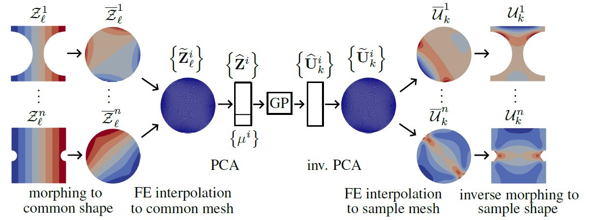Figure 1: MMGP inference workflow for fields outputs

1. Load configuration

The configuration yaml file is loaded, as well as the problem definition from the PLAID format. These setting are then printed to the console.

from mmgp.utils import read_configuration, read_problem, print_setting

configuration = read_configuration(config_file="configuration.yaml")
problem = read_problem(configuration)
print_setting(configuration, problem)

*********************** Configuration **********************
case_name                : SimpleTest
init_dataset_location    : ../../../examples/SimpleTest/input_data
generated_data_folder    : data
zone_name                : Zone
base_name                : Base_2_2
train_set                : train
test_set                 : test
common_mesh_index        : 3
verbose                  : False
morphing                 :
      algo    : Floater
      options : None
dimensionality_reduction :
      input_coord_fields  :
            algo    : SnapshotPOD
            options :
                  number_of_modes  : 2
                  correlation_type : mass_matrix
      output_coord_fields :
            algo    : SnapshotPOD
            options :
                  number_of_modes  : 2
                  correlation_type : mass_matrix
regression               :
      reference_regressor        : 0
      uncertainties              : True
      number_Monte_Carlo_samples : 10
      algo                       : mmgp.backends.scikit_learn
      options                    :
            kernel         : Matern
            kernel_options :
                  nu : 2.5
            optim          : fmin_l_bfgs_b
            num_restarts   : 2
            anisotropic    : True
            show_warnings  : False
******************** Problem definition ********************
split names          : ['train', 'test']
input scalar names   : ['a']
output scalar names  : ['l']
output field names   : ['field_1', 'field_2']

TODO: continue the list

• init_dataset_location indicates where the dataset in PLAID format is located, containing the definition of the learning problem, and all the samples, each contain a physics configuration (see Figure 2).

• generated_data_folder is the location of the folder where the MMGP method will save the produced data. Here, it a the dolfer data in the current working director.

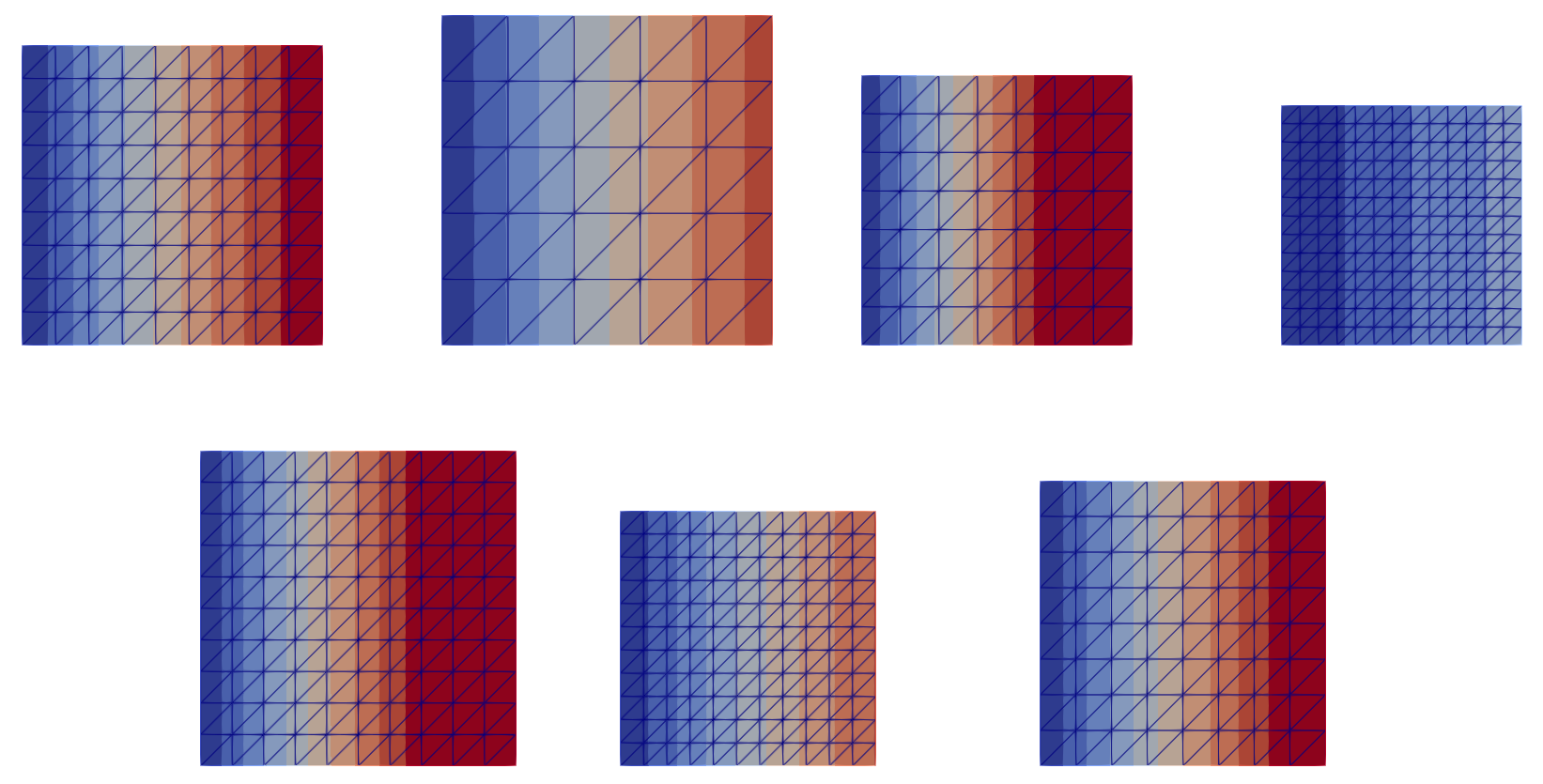Figure 2: Initial database, representation of field_1; (top) training set, (bottom) testing set. We notice a variety of shape and meshes sizes, as well as fields magnitudes

If we inspect the current working directory, it contains only the configuration.yaml file and the present notebook:

import os
os.listdir()

['configuration.yaml', 'notebook.ipynb']

2. Preprocess database

The following pre_process function morphs the meshes $\mathcal{M}^i$ of all samples onto the common mesh $\overline{\mathcal{M}}_c$ of the reference shape $\overline{\Omega}$ and computes finite element interpolations on it. The morphing algorithm is chosen following the configuration morphing\algo from the configuration.yaml file, with provided options.

The folder data is created and populated with three folders (see Figure 1):

• FEInterpolationOperators: precomputation of finite element interpolation operators between each sample mesh and the common mesh of the reference shape, both direct and inverse,

• SimpleTest_morphed: dataset with morphed meshes $\overline{\mathcal{M}}^i$ and transported fields $\overline{\mathcal{Z}}^i_{\ell}$ and $\overline{\mathcal{U}}^i_k$ (see Figure 3),

• SimpleTest_morphed_and_projected: dataset all fields $\widetilde{\mathbf{Z}}^i_{\ell}$ and $\widetilde{\mathbf{U}}^i_k$ interpolated onto the common mesh $\overline{\mathcal{M}}_c$ (see Figure 4).

from mmgp.preprocessing import pre_process

pre_process(configuration)
os.listdir("data")

Kokkos::OpenMP::initialize WARNING: OMP_PROC_BIND environment variable not set
  In general, for best performance with OpenMP 4.0 or better set OMP_PROC_BIND=spread and OMP_PLACES=threads
  For best performance with OpenMP 3.1 set OMP_PROC_BIND=true
  For unit testing set OMP_PROC_BIND=false

['FEInterpolationOperators',
 'SimpleTest_morphed_and_projected',
 'SimpleTest_morphed']

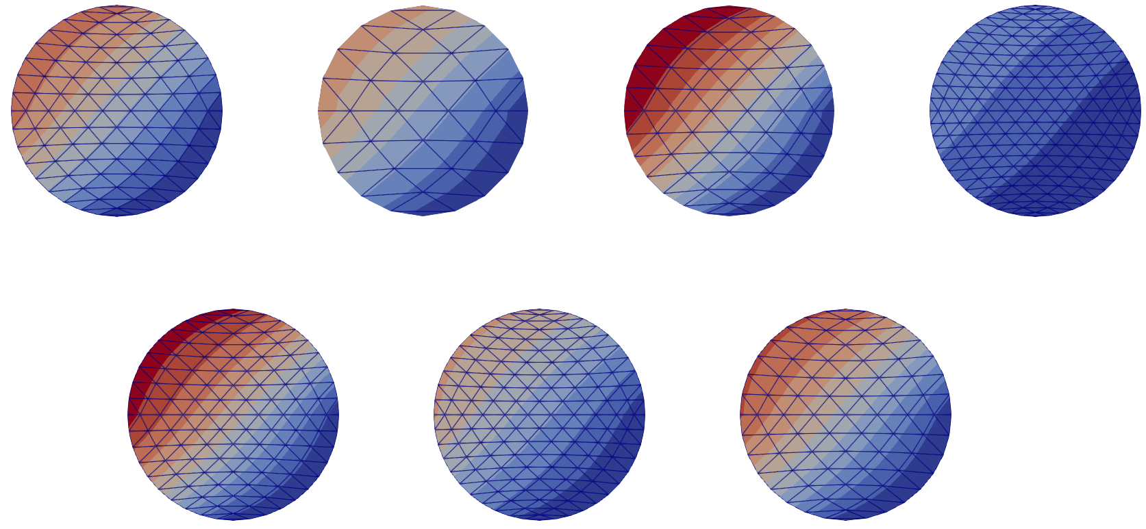Figure 3: Morphed database, representation of field_1; (top) training set, (bottom) testing set. The meshes $\mathcal{M}^i$ have been morphed, and the fields transported. The morphed meshes $\overline{\mathcal{M}}^i$ are discretization of the same reference shape (the unit disk $\overline{\Omega}$), but are still different

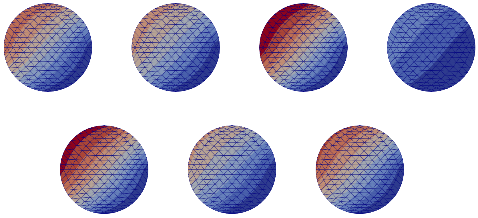Figure 4: Morphed and interpolated database, representation of field_1; (top) training set, (bottom) testing set. The fields have been interpolated onto the common mesh $\overline{\mathcal{M}}_c$ of the reference shape $\overline{\Omega}$

3. Train

The following train function trains the Gaussian process regressor using data from the training set. The GP algorithm is chosen following the configuration regression\algo from the configuration.yaml file, with provided options. The inputs and outputs of the GP are taken from the problem_definition of the init PLAID object. The dimensionality of the fields input and output interpolated on the common mesh $\overline{\mathcal{M}}c$, respectivement $\widetilde{\mathbf{Z}}^i{\ell}$ and $\widetilde{\mathbf{U}}^i_k$, is reduced in this stage to obtain $\widehat{\mathbf{Z}}_{\ell}$ and $\widehat{\mathbf{U}}^i_k$, following the configurations dimensionality_reduction\algo from the configuration.yaml (see Figure 1).

The file trainingRegressionData.pkl is added in the folder data to save the trained GP and corresponding scalers.

from mmgp.processing import train

train_data = train(configuration, problem)
os.listdir("data")

['FEInterpolationOperators',
 'SimpleTest_morphed_and_projected',
 'SimpleTest_morphed',
 'trainingRegressionData.pkl']

4. Infer

The following infer function computes the prediction using the trained GP, for both the training and testing data.

The file allPredictedData.pkl is added in the folder data to save the predicted data.

from mmgp.processing import infer

predicted_data = infer(configuration, problem)
os.listdir("data")

['allPredictedData.pkl',
 'FEInterpolationOperators',
 'SimpleTest_morphed_and_projected',
 'SimpleTest_morphed',
 'trainingRegressionData.pkl']

5. Compute metrics

The following compute_metrics function computes rRMSE and R2 for all output scalars and fields, for both the training and testing data.

from mmgp.postprocessing import compute_metrics

metrics = compute_metrics(configuration, problem)

import rich
rich.print(metrics)

{
    'rRMSE for fields': {
        'train': {'field_1': '0.00197519', 'field_2': '0.00197519'},
        'test': {'field_1': '0.0584740', 'field_2': '0.0584740'}
    },
    'rRMSE for scalars': {'train': {'l': '3.68813e-07'}, 'test': {'l': '8.14948e-05'}},
    'R2 for fields': {
        'train': {'field_1': '0.999981', 'field_2': '0.999981'},
        'test': {'field_1': '0.972894', 'field_2': '0.972894'}
    },
    'R2 for scalars': {'train': {'l': '1.00000'}, 'test': {'l': '0.999999'}}
}

6. Export predictions

The following export_predictions saves the predicted data on disk in the PLAID format.

The folder SimpleTest_predicted is added in the folder data.

from mmgp.postprocessing import export_predictions

predicted_dataset = export_predictions(configuration, problem)
os.listdir("data")

['SimpleTest_predicted',
 'allPredictedData.pkl',
 'FEInterpolationOperators',
 'SimpleTest_morphed_and_projected',
 'SimpleTest_morphed',
 'metrics.yaml',
 'trainingRegressionData.pkl']